ClickHouse MergeTree: Parts, Merges, and the Meaning of "Primary Key"
 .
A walk from the storage engine up to the vocabulary. The throughline: almost every surprising thing about ClickHouse — why it batches inserts, why dedup is eventual, why a skip index can't save a bad key, why "primary key" doesn't mean what a Postgres user thinks — falls out of one design choice: data lives as immutable, sorted parts that merge in the background. Get that, and the rest is consequence.
.
A walk from the storage engine up to the vocabulary. The throughline: almost every surprising thing about ClickHouse — why it batches inserts, why dedup is eventual, why a skip index can't save a bad key, why "primary key" doesn't mean what a Postgres user thinks — falls out of one design choice: data lives as immutable, sorted parts that merge in the background. Get that, and the rest is consequence.
What ClickHouse Is
ClickHouse is an open-source, column-oriented database built for OLAP — scanning and aggregating billions of rows in milliseconds to low seconds. Data is stored by column (so a query reads only the columns it touches, and similar values compress hard), executed in vectorized blocks (SIMD-friendly, conceptually the same shape as Polars/DataFusion over Arrow batches), and distributed shared-nothing with replication coordinated by Keeper, its Raft-based ZooKeeper replacement.
Against BigQuery, the mental model is: BQ is a fully-managed serverless warehouse where storage and compute are decoupled and someone else runs everything; ClickHouse is a specialized columnar engine you operate yourself (or via ClickHouse Cloud), trading that operational burden for very low latency at high concurrency and real-time ingest. It's OLAP-first — weaker on frequent updates/deletes, heavy multi-table joins, and transactional guarantees.
The heart of it all is the MergeTree engine family.
The Storage Hierarchy: Partition → Part → Granule
These three levels get conflated constantly, and keeping them straight resolves most confusion. Note especially: the 8,192 figure is the granule, not the part. A part can hold millions of rows.
- Partition — a logical group of parts sharing a
PARTITION BYvalue (e.g. one month). Coarse; mostly a data-lifecycle tool (drop/TTL old partitions). Merges never cross a partition boundary. Over-partitioning is an anti-pattern — don't partition by anything high-cardinality. - Part — a directory on disk: one compressed file per column, marks files mapping granules to byte offsets, the sparse
primary.idx, checksums, and a minmax index for partition pruning. This is the unit that gets merged. One partition typically holds many parts. - Granule — ~8,192 rows inside a part (
index_granularity); the unit the sparse index points at and the smallest block read off disk. One part contains many granules.
So: one partition → many parts → each part → many granules.
[!info] The 8,192 clarification
index_granularity = 8192is the number of rows between marks in the sparse index, i.e. the granule size — not a limit on part size. The sparse "primary index" stores one entry per granule (the key-tuple values at its boundary), so the index for a billion-row table is a few MB and lives in RAM.
Parts and the MergeTree Lifecycle
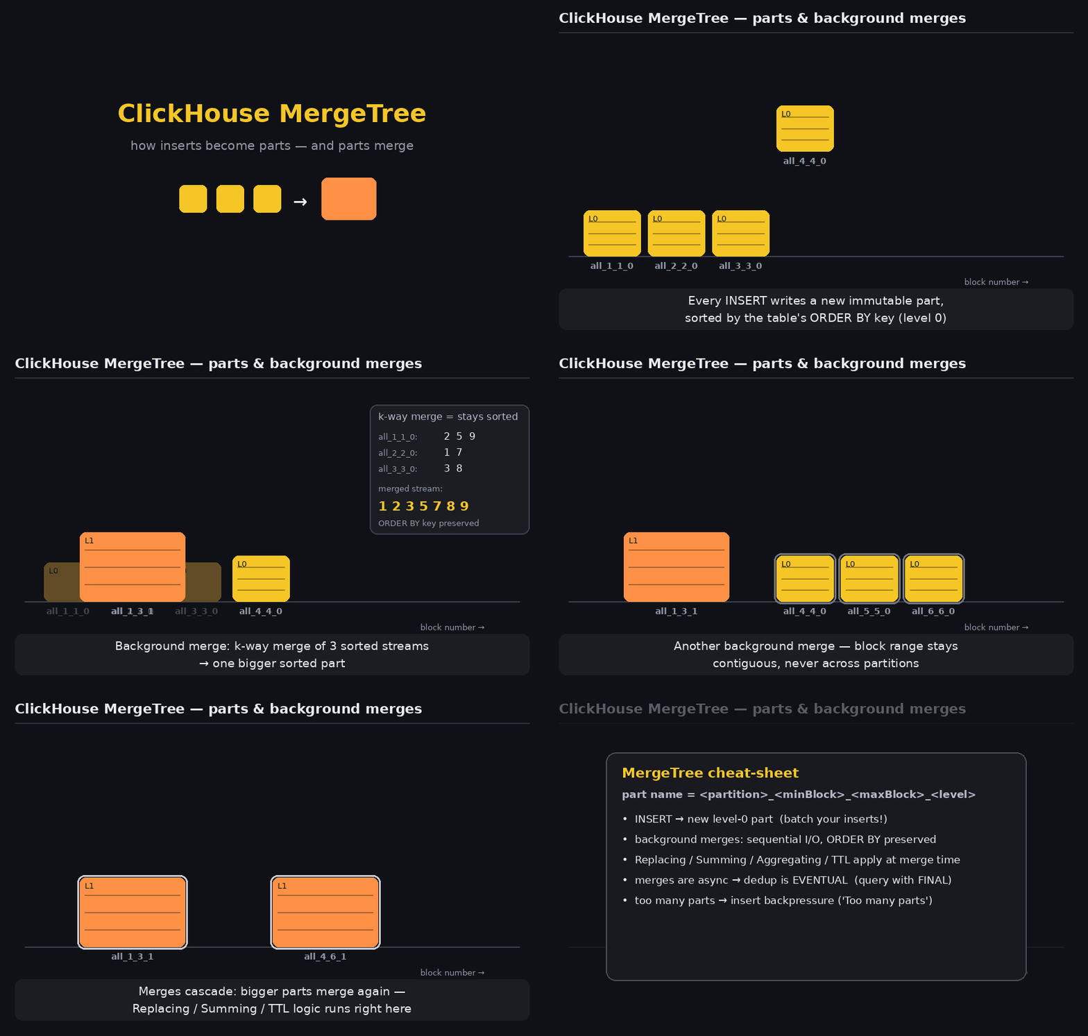
Every INSERT writes a new immutable part, its rows sorted by the table's ORDER BY key, at merge level 0. Background threads then continually merge small parts into larger ones, LSM-style. This is exactly why ClickHouse wants batched inserts (thousands of rows, or async_insert) — row-at-a-time writes cause a part explosion.
The part name encodes lineage: partition_minBlock_maxBlock_level. Each insert takes the next block number at level 0; merging the parts covering blocks 1–3 produces all_1_3_1. (Mutations append a mutation version.) Small parts are written compact (all columns in one file) and flip to wide (file-per-column) past a size threshold, usually at their first merge.
The animation below shows the whole cycle — inserts landing as level-0 parts, the scheduler selecting neighbours, the k-way merge preserving sort order, old parts going inactive, and merges cascading upward:
Mechanically a merge is a k-way merge of already-sorted streams: sequential reads, one sequential write, ORDER BY preserved, data recompressed into larger and better-compressing blocks. It's also the hook where engine semantics run — ReplacingMergeTree keeps the newest row per key, Summing/AggregatingMergeTree fold or aggregate, CollapsingMergeTree cancels ±1 sign pairs, TTL rules drop rows or move parts across storage tiers, and lightweight-delete masks get physically applied.
[!warning] Merge semantics are eventual Merges are asynchronous and never guaranteed complete, so dedup/aggregation is eventual. At query time you either pay for
FINAL, useargMax/GROUP BYpatterns, or forceOPTIMIZE TABLE … FINAL(expensive — it rewrites everything). Under replication the merge is logged through Keeper: one replica executes it, the others fetch the resulting part.
How Merges Choose Which Parts to Combine
Partition is the filter, not the whole answer. Selection needs two conditions together:
- Same partition — merges never cross a
PARTITION BYboundary. - Contiguous in the block-number sequence — every active part covers a non-overlapping
minBlock_maxBlockrange, and these ranges are totally ordered. "Adjacent" means neighbouring in that ordering, with no active part in between. You can mergeall_1_3+all_4_6(they touch), but notall_1_3+all_7_9whileall_4_6still sits between them.
On top of that the scheduler adds a desirability heuristic: it prefers parts of similar size (to limit write amplification) and caps the merged result (roughly 150 GB by default), above which parts are left alone. So it isn't strictly left-to-right — it picks the cheapest contiguous run of similar-sized neighbours.
Why contiguity is required: keeping merges to adjacent block ranges means the result still covers one clean interval, so parts always tile the block space without overlap. That's the invariant the whole engine leans on — an ordered set of non-overlapping sorted runs. Push inserts faster than merging can keep up and you hit "Too many parts" backpressure (delayed inserts, then rejections) — the real engineering reason behind batching.
The Sort Key: ORDER BY
Within every part, rows are physically sorted by the full tuple of ORDER BY columns, lexicographically — first column, then ties broken by the second, then the third. Same as a multi-level spreadsheet sort. With ORDER BY (tenant, device_id, ts):
tenant  device_id  ts
A       d1         09:00
A       d1         09:05    ← same tenant+device → ordered by ts
A       d2         08:55    ← device_id breaks the tie *before* ts matters
A       d2         09:10
B       d1         08:00    ← new tenant starts a fresh ordering
A/d2/08:55 sits below A/d1/09:05 despite the earlier timestamp, because device_id is compared first. It's one sorted run over the tuple, not separate per-column sorts — which is exactly what makes merges the cheap k-way interleave shown above.
The prefix rule. Primary-index pruning only works on a leading prefix of the key. With ORDER BY (tenant, ts): filtering on tenant, or tenant AND ts, prunes granules; filtering on ts alone does not (you'd need a skip index or a projection). So column order is the real decision — put the column you filter on most first. General guidance: low cardinality before high cardinality, so sorted runs stay long, the exclusion search stays effective, and compression improves. For time-series the timestamp usually goes last. (Exception: heavily repeated attributes like clickstream can justify leading with a higher-cardinality column purely for compression/locality.)
ORDER BY vs PRIMARY KEY — the Decoupling Lever
By default PRIMARY KEY equals ORDER BY and the distinction is invisible. But they can differ, with one constraint: PRIMARY KEY must be a prefix of ORDER BY. This separates two jobs that otherwise get fused:
ORDER BY→ how rows are physically sorted (drives compression + range locality).PRIMARY KEY→ which columns are materialized into the in-memory sparse index.
ORDER BY    (tenant, device_id, ts)
PRIMARY KEY (tenant, device_id)
Data is sorted by all three; the index only carries the first two. Handy when a trailing high-cardinality column (a millisecond timestamp) would bloat the index without helping pruning. The governing fact: extra columns in the primary key do not slow down SELECT, but a long primary key does hurt insert performance and memory (each granule mark stores the full key tuple in RAM).
[!tip] The lever BigQuery doesn't give you A long
ORDER BYfor sort locality and compression, carrying a shortPRIMARY KEYprefix for a lean index — decoupling how finely sorted from how big the index. In BQ the clustering columns are unavoidably both the sort order and the pruning metadata; you can't split them.
The BigQuery Analogy (and Where It Leaks)
The mapping is clean and worth internalising:
| BigQuery | ClickHouse | Shared behaviour |
|---|---|---|
CLUSTER BY | ORDER BY | Compound, lexicographic, prefix rule (filter left-to-right) |
| Partitioning column | PARTITION BY | Coarse pruning dimension |
| Automatic re-clustering | Background merges | A free background process that repairs sort order after writes |
Both cluster keys sort data so filtered scans skip storage units; both degrade as new data arrives and are repaired automatically. But three real divergences:
1. Column limit. BigQuery hard-caps clustering at 4 columns (top-level, non-repeated, of a supported type). ClickHouse has no explicit limit — practically 3–5 is the sweet spot; the creator has mentioned seeing ~20 in a SummingMergeTree case but doesn't recommend it. The cap difference traces straight to the sparse index: in ClickHouse the ceiling is a soft insert-cost/memory tradeoff, not a schema rule.
2. Index exposure. ClickHouse's ORDER BY doubles as the sparse primary index you can reason about and tune; BQ clustering exposes no user-visible index, just block-level min/max metadata.
[!warning] Gotcha when porting BQ intuition — cardinality inverts BigQuery clustering is happy leading with high-cardinality columns (and even benefits from them). ClickHouse wants low-cardinality columns first — better generic-exclusion search and better compression — with the high-cardinality column (usually the timestamp) trailing. Copying a BQ
CLUSTER BYorder directly into a ClickHouseORDER BYcan quietly kill pruning.
Why It's Called "Primary Key"
The term has two independent lineages that merely share the word primary, and ClickHouse uses the older, storage-layer one:
- Relational (Codd, 1970): a logical constraint — a candidate key guaranteeing row uniqueness and identity. The meaning most people carry.
- Physical storage: the primary index — the principal index dictating how rows are laid out on disk, i.e. a clustered index. "Primary" here means first-order / principal, as opposed to secondary indexes.
ClickHouse means the second, and its own taxonomy makes that explicit: the sparse mark index built from PRIMARY KEY is the primary index, while minmax / set / bloom-filter skip indexes are literally the secondary indexes. So PRIMARY KEY names "the key backing the primary index" — primary as opposed to secondary, nothing to do with uniqueness.
It isn't a rogue choice: InnoDB and SQL Server already overload the term the same way — there the primary key is the clustered index and sets physical row order. ClickHouse kept that half (organise and sort the data) and dropped the other half (enforce uniqueness). It dropped uniqueness deliberately: a uniqueness check means a read on every insert, incompatible with cheap, batched, append-only writes into immutable sorted parts. Arguably ClickHouse uses "primary" more literally than a typical RDBMS — the first-order key by which data is primarily arranged. It only feels wrong because OLTP made the constraint meaning dominant.
[!note] Not a uniqueness constraint ClickHouse's
PRIMARY KEYenforces nothing about uniqueness or non-null. It's the organising/index key — closer to a SQL Server clustered index than to a relational primary key. This is also why it maps onto BQ's clustering key rather than onto the RDBMS notion.
Primary vs Secondary Indexes — a Strict Hierarchy
This axis (principal vs auxiliary) is the whole logic, and it's load-bearing, not cosmetic:
- The primary index is the data. It's the sort order rows physically live in — not a separate structure pointing at rows, just marks describing where you already are in the sorted stream. Exactly one exists (you can't sort a deck two ways at once). Zero redundancy.
- Secondary (skip) indexes are auxiliary metadata about blocks — per-granule minmax,
set, bloom filters. They reorder nothing; they let you skip granules the primary order didn't already cluster for you. Optional, many allowed, and they only help when the indexed column correlates with the primary order — otherwise the values are smeared across granules and the index prunes nothing while still adding overhead.
The crux: a secondary index cannot rescue a bad primary-key choice, because it rides on top of the physical layout the primary key already dictated. This is the opposite of a row-store like Postgres, where an independent secondary B-tree can rescue almost any query with its own sorted pointer structure. In a columnar sorted-parts world the primary key is genuinely primary — everything else refines it, never replaces it.
Hence the escalation ladder:
- Get
ORDER BYright first. It's the single highest-leverage schema decision. - Reach for projections — essentially a second physical copy of the data sorted differently, maintained on insert. The real escape hatch when you need a genuinely different access path.
- Skip indexes last — a correlated tie-breaker, not a rescue.
Key Takeaways
- Immutable sorted parts + background merges is the one idea everything else derives from.
- Partition ⊃ Part ⊃ Granule. 8,192 rows is the granule (the sparse-index stride), not the part.
- Batch your inserts — row-at-a-time causes part explosion and "Too many parts" backpressure.
- Merge selection = same partition + block-range contiguity + size-similarity, capped ~150 GB. Contiguity keeps parts tiling the block space with no overlap.
- Merge-time semantics (Replacing/Summing/Aggregating/TTL) are eventual — use
FINALorargMax/GROUP BYat read time. ORDER BYis a compound lexicographic sort; pruning needs a leading prefix. Column order is the real decision; low-cardinality generally goes first.- Split
ORDER BY(long, for sort/compression) fromPRIMARY KEY(short, for a lean index) — a lever BQ lacks. Extra key columns don't slowSELECT, only inserts/memory. - BQ
CLUSTER BY≈ CHORDER BY, but: BQ caps at 4 columns / CH has no limit; CH exposes the sparse index; cardinality ordering inverts. - "Primary key" = primary index (clustered), not a uniqueness constraint — primary as opposed to secondary. Uniqueness was dropped because it needs a read per insert.
- A skip index can't fix a bad
ORDER BY. Escalate:ORDER BY→ projections → skip indexes.
References
- MergeTree table engine — ClickHouse Docs
- The definitive guide to ClickHouse query optimization
- Picking ORDER BY / PRIMARY KEY / PARTITION BY — Altinity KB
- Introduction to clustered tables — BigQuery Docs
- Create clustered tables — BigQuery Docs
react & discuss
EOF · cd ~